GPU Memory Requirements for LLMs

GPU memory budget divided among model weights, KV cache, runtime overhead and operating headroom

GPU memoryLLM sizingKV cacheVRAMAI inferencemixture of experts

In brief

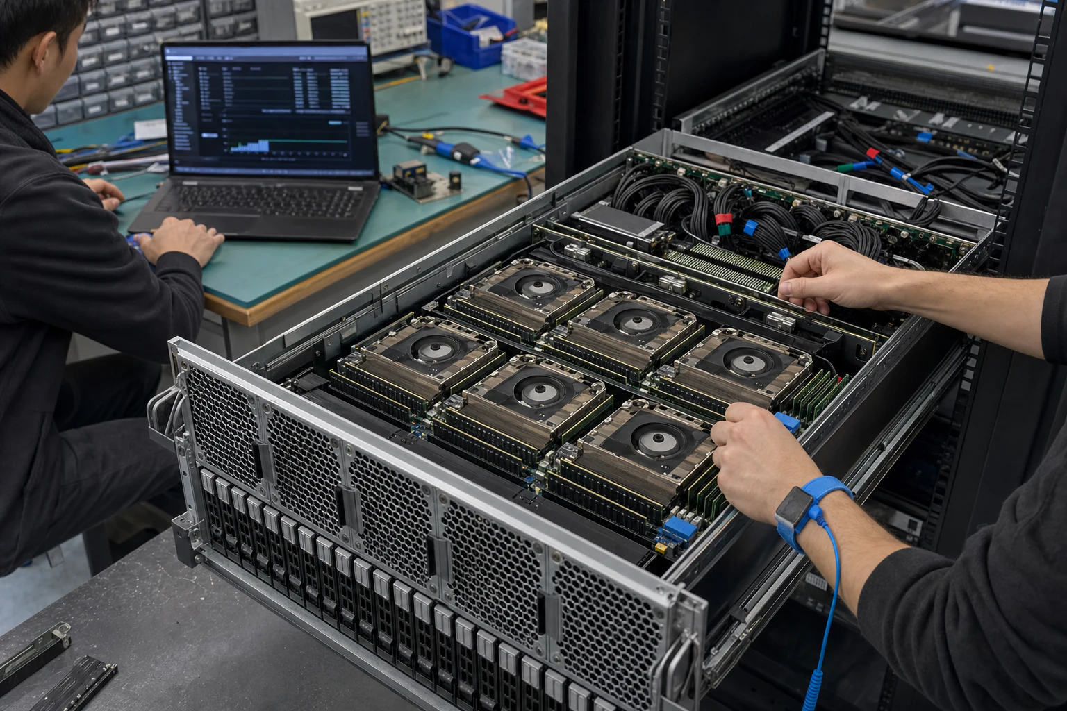
Start LLM GPU-memory sizing with the nominal weight payload: approximately 2 GB per billion parameters at FP16 or BF16, 1 GB per billion at 8-bit, and 0.5 GB per billion at 4-bit. Verify the exact checkpoint footprint, then add KV cache for the target context and concurrency, serving-framework allocations, and safety headroom. A model that merely loads is not yet a production service.

Key takeaways

Model weights provide the fixed memory floor: parameter count multiplied by the selected storage precision.
KV-cache demand grows with sequence length and simultaneous requests, so long-context high-concurrency serving can consume substantial additional memory.
A mixture-of-experts model normally needs all expert weights resident; active parameters describe per-token compute, not total weight memory.
Per-node memory determines whether a model can stay inside one server or requires multi-node tensor or expert parallelism.
Arithmetic produces a shortlist; final fit, quality, throughput, and latency require validation on the exact checkpoint and serving stack.

GPU memory sizing has three layers. Model weights form the fixed floor. KV cache changes with the live workload. Runtime allocations and safety headroom complete the budget. Skipping either of the last two is how a configuration that loads successfully becomes a service that fails under real context or concurrency.

The calculation also shapes topology. If the complete budget fits inside one node, the deployment avoids adding scale-out networking to the model-parallel critical path. If it does not, the serving design must distribute the model and account for the resulting interconnect and operational cost.

Calculate the Model-Weight Floor

For a conventional dense checkpoint, the first estimate is:

nominal weight payload (bytes) = total parameters × stored bits per parameter ÷ 8

Using decimal units, one billion parameters needs approximately 2 GB at 16-bit, 1 GB at 8-bit, or 0.5 GB at 4-bit.

Stored precision	Approximate bytes per parameter	7B weights	70B weights	400B weights
FP16 / BF16	2	14 GB	140 GB	800 GB
FP8 / INT8	1	7 GB	70 GB	400 GB
4-bit class	0.5	3.5 GB	35 GB	200 GB

These are planning estimates, not exact checkpoint sizes or allocated-memory results. GB in this table is decimal; one GiB is 1,073,741,824 bytes. Model files can include metadata, tied or untied tensors, and packing overhead. Quantised checkpoints commonly retain some tensors at higher precision and store scales or zero points. A runtime may also materialise converted or temporary representations.

Precision also affects more than capacity. Moving from BF16 to FP8 or 4-bit can change supported kernels, throughput, and output quality. The quality effect is model- and task-specific. A quantised model that performs well for summarisation may behave differently on code, hard reasoning, legal drafting, or a domain-specific extraction task.

The correct sequence is to calculate the saving, then validate quality on the actual tasks. Do not treat a lower bit count as a free capacity upgrade.

Add KV Cache for Context and Concurrency

During autoregressive generation, a transformer reuses attention keys and values calculated for earlier tokens. The serving system stores them in a key-value cache so it does not recompute the complete sequence for every new token.

KV-cache memory grows along several dimensions:

Number of transformer layers.
Number of key-value heads and each head’s dimension.
Bytes used for cache elements.
Tokens retained in each active sequence.
Number of simultaneous sequences.

A simplified estimate for a conventional decoder-only attention model is:

KV-cache bytes per sequence = 2 × cached attention layers × KV heads × head dimension × bytes per cache element × cached tokens

The first factor of two represents keys and values. The formula is a model-wide logical total before any tensor-parallel placement. Multi-latent attention, sliding-window attention, hybrid attention/SSM models, cross-attention, cache quantisation, and layer-specific layouts need architecture-aware treatment. Use the serving framework’s model-specific estimator as a starting point and runtime profiling as the final evidence.

An illustrative calculation

Consider a 70B-class model with 80 layers, 8 KV heads, head dimension 128, and a 16-bit cache:

2 × 80 × 8 × 128 × 2 bytes = 327,680 bytes per cached token

That is 0.3125 MiB per cached token. A fully occupied 32,000-token sequence would therefore use 10.49 GB, or 9.77 GiB, of KV cache. Ten such sequences would use about 97.7 GiB before allocator and block-granularity effects.

This is deliberately illustrative. Real requests have different sequence lengths, may share prefixes, may not fill the configured maximum context, and may use different cache precision. Model architectures also differ. The example shows the shape of the risk: retained prompt and generated tokens, multiplied by concurrency, can make cache memory comparable with the model weights.

Serving frameworks can manage or reduce cache demand through paged allocation, shared prefixes, lower-precision cache formats, and scheduling. PagedAttention, introduced by Kwon et al., stores cache data in blocks rather than reserving a worst-case contiguous allocation for every sequence. That reduces allocation waste, but it does not make the live tokens’ cache payload disappear.

Build a Complete Serving Memory Budget

A production estimate needs four explicit budget blocks:

Budget block	Behaviour	How to estimate it	Validation evidence
Model weights	Mostly fixed after checkpoint and precision are selected	Sum actual tensor storage, with parameter arithmetic as a cross-check	Runtime-reported allocated weights
KV cache	Variable with context, concurrency, architecture, and cache precision	Framework estimator plus representative request profiles	Cache utilisation under load
Runtime and temporary memory	Changes with kernels, batching, graphs, and framework	Framework guidance and observed peak allocation	Peak allocated and reserved memory
Safety and operational headroom	Protects against fragmentation, growth, and workload variation	Explicit percentage or reserved capacity policy	Load test without out-of-memory events

Do not allocate every available byte to the advertised maximum workload. Production headroom is needed for request variation, software changes, health checks, and operational recovery. The policy should state what happens when the service approaches the memory limit: reject, queue, shorten context, route to another node, or scale capacity.

Mixture-of-Experts: Total and Active Parameters

Mixture-of-experts models commonly report two parameter counts: total parameters and the subset activated for a token.

The active count describes the experts selected for that token and therefore helps explain compute per token. It does not normally reduce the complete resident weight set to the active count. The router can select different experts for later tokens, so all expert weights normally need to be resident in aggregate across the participating accelerators. Deliberate expert or CPU offload is possible in some stacks, but its transfer cost must be measured.

The sizing rule is:

Use total parameters for the base weight-memory estimate.
Use active parameters and architecture to reason about per-token compute.
Use the official model card and serving implementation to identify any exceptions or placement constraints.

MoE can provide capability and throughput advantages relative to a dense model with a similar total parameter count. It should not be sold as though inactive experts require no memory.

Worked Capacity Scenarios

Model-family labels age quickly and can hide material differences between revisions. The following checkpoint-neutral scenarios isolate the weight arithmetic. They are hypothetical capacity examples, not claims about a named model or a supported deployment.

Planning scenario	Total / active parameters	Nominal BF16 weights	Nominal 8-bit weights	Nominal 4-bit weights
Dense model	70B / not applicable	140 GB	70 GB	35 GB
MoE scenario A	400B / 20B	800 GB	400 GB	200 GB
MoE scenario B	700B / 40B	1,400 GB	700 GB	350 GB
Very large MoE scenario	1.6T / 50B	3.2 TB	1.6 TB	800 GB

Now compare those weight floors with two 8-GPU capacity classes: 8 × 288 GB, or 2,304 GB total, and 8 × 192 GB, or 1,536 GB total. At a nominal one byte per parameter, the 1.6T scenario needs 1,600 GB and therefore cannot fit in the 1,536 GB aggregate. It clears the 2,304 GB aggregate arithmetically, leaving 704 GB before KV cache, runtime allocations, placement imbalance, and safety headroom.

The 700B scenario illustrates a subtler trap. Its nominal BF16 weights are 1,400 GB, just below 1,536 GB, but the remaining 136 GB is unlikely to constitute a defensible production budget without a measured, unusually light request profile. By contrast, its nominal 8-bit weight floor is 700 GB. Whether that precision is usable depends on an exact quantised checkpoint, supported kernels, and task-level quality tests.

From weight fit to service fit

Consider a separate, hypothetical 70B deployment. The selected 8-bit checkpoint occupies 72 GB after its higher-precision tensors and quantisation metadata are counted. The model uses the KV layout from the earlier example, and the service must sustain 16 simultaneous sequences with an average of 8,000 retained tokens. A profile run records 18 GB of peak runtime and temporary allocations.

Budget item	Example amount	Basis
Loaded checkpoint tensors	72.00 GB	Measured for the selected deployment artifact
KV cache	41.94 GB	327,680 bytes × 8,000 tokens × 16 sequences
Runtime and temporary allocations	18.00 GB	Peak observed in a representative profile run
Service-allocation subtotal	131.94 GB	Sum before operational reserve
Minimum installed capacity at a 20% free-memory policy	164.93 GB	131.94 GB ÷ 0.80

On capacity arithmetic alone, a 192 GB accelerator clears that policy: the example allocations leave about 60 GB free. That still is not an acceptance result. The 16-sequence average can conceal a heavier p95 tail, the framework may reserve memory differently under sustained batching, and a later software version may change graph or workspace allocations. The team should replay the planned request distribution and confirm both peak memory and service latency.

This example also shows why units and evidence types should stay visible. The weight value is measured, the KV value is calculated from an architecture, the runtime value is profiled, and the reserve is an operating policy. Treating all four as the same kind of estimate makes review and troubleshooting harder.

Several details can change the conclusion:

Published checkpoints may store a different precision from the deployment target.
A framework may not support the desired quantisation or kernels on the selected accelerator.
Tensor-parallel placement can introduce per-device imbalance or replicated allocations.
Long contexts and high concurrency can consume the apparent remaining memory.
Memory totals are aggregate capacities; topology determines whether the runtime can use them as assumed.

The arithmetic is valuable for shortlisting. It is not acceptance evidence.

What the Memory Math Means for Hardware

Per-GPU and per-node memory determine whether the model can remain inside one server. A single-node deployment can simplify latency, cabling, orchestration, and failure analysis because model-parallel traffic stays within the platform’s local GPU fabric.

When the complete budget does not fit, common options include:

Use a validated lower-precision checkpoint.
Select a smaller model and test whether it meets the quality bar.
Distribute the model across GPUs or nodes using tensor, pipeline, or expert parallelism.
Reduce context or concurrency requirements.
Separate workload classes across model sizes.

Multi-node serving is a valid architecture, not a failure. It adds network communication to the model path, more failure domains, distributed scheduling, and a larger operating surface. The data-centre fabric, NICs, switches, optics, congestion behaviour, telemetry, and recovery plan become part of the inference result.

CPU or storage offload can allow a model to run when accelerator memory is insufficient, but moving weights over a slower path generally changes latency and throughput substantially. Treat offload as a measured architecture, not a substitute for adequate production memory.

A Five-Step Sizing Worksheet

1. Fix the exact checkpoints

Record model publisher, repository, revision, architecture, total and active parameters, licence, and supported context. A model family name is not enough.

2. Select and validate precision

Calculate the weight floor at the candidate precision. Run representative quality tests before using a lower-precision result as a procurement assumption.

3. Model the live request profile

Record typical, p95, and maximum prompt and output lengths, concurrent sequences, request rate, prefix reuse, multimodal inputs, and the target latency. Use the serving framework’s model-specific cache estimator.

4. Add runtime and safety headroom

Include framework allocations, temporary buffers, batching, graph capture, fragmentation, monitoring, software changes, and a documented headroom policy.

5. Compare topology and validate

Compare the complete budget with both the per-rank capacity and the node aggregate. Shortlist single-node and distributed options, then measure model load, peak memory, time to first token, output rate, aggregate throughput, p95 latency, and out-of-memory behaviour under the planned request mix.

Worksheet output	Decision it supports
Exact model and precision	Weight-memory floor and quality gate
Context and concurrency profile	KV-cache requirement
Runtime and headroom allowance	Safe usable node capacity
Single-node fit	Simpler local topology option
Distributed fit	Network and orchestration requirements
Measured load test	Final acceptance or rejection

Where the Formulas Stop

Memory arithmetic does not predict user capacity. Throughput and latency depend on prompt-to-output ratio, batching, scheduler policy, kernels, framework version, hardware topology, storage, network, and the latency target.

It also does not decide whether a model is useful. A smaller model that passes the workload evaluation can be a stronger system choice than a larger model that increases memory, latency, energy, and operating complexity without improving accepted outcomes.

Use the calculation to produce a defensible shortlist. Use an exact checkpoint, fixed test conditions, and measured service objectives to make the final decision.

The network and storage planning guide shows how memory-driven node topology affects the rest of the private AI system, while the private AI procurement scorecard provides a buyer-facing evidence framework.

Product fit

Where xSONiC Fits

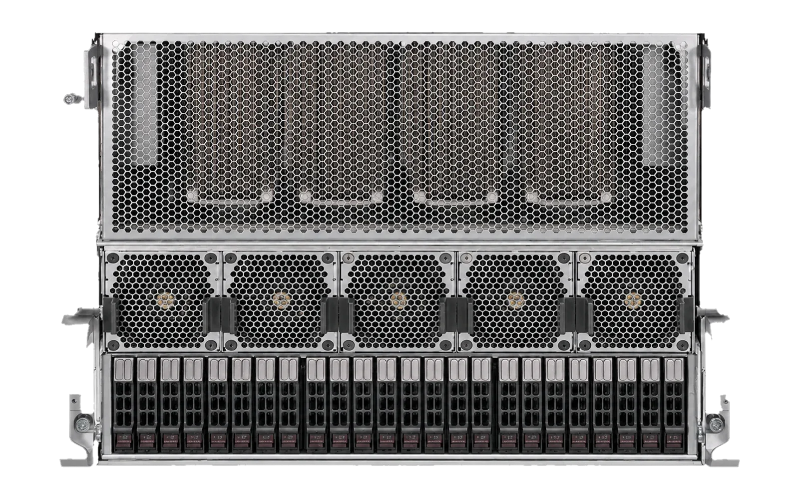
The xSONiC AI Inference Server provides 8-GPU MI355X and MI300X platform options. xSONiC sizes the node from the exact checkpoint, precision, context, concurrency, serving framework, network, and storage plan, then validates memory headroom and service performance before handover.

ai infrastructurexSONiC AI Inference ServerPrivate AI inference platform for local LLM, RAG, coding, document intelligence, and multimodal services, with xSONiC deployment support across compute, network, storage, and validation.View product

FAQ

Frequently asked questions

How much GPU memory is needed for a 70B model?

The nominal weight payload is approximately 140 GB at 16-bit, 70 GB at 8-bit, or 35 GB at 4-bit using decimal units. Quantisation metadata and mixed-precision tensors can increase the actual footprint. Add KV cache, runtime allocations, batching headroom, and a safety margin before selecting the GPU configuration.

Does a mixture-of-experts model need memory only for its active parameters?

Normally no. The router may select different experts for different tokens, so the complete expert weight set must remain resident or reachable. Active parameters indicate approximate compute per token, while total parameters drive the base weight-memory requirement.

How much memory does the KV cache use?

It depends on model architecture, cache precision, sequence length, and concurrent sequences. Use the exact serving framework's estimator and validate representative prompts because a generic per-token number does not transfer safely between models.

Can an LLM be split across multiple GPUs or servers?

Yes. Tensor, pipeline, and expert parallelism can distribute a model, but they add interconnect traffic, orchestration, failure domains, and latency considerations. Compare those costs with a higher-memory single-node configuration and validate both against the service target.

Primary sources and standards

First-party documentation, standards, and official technical references used to support specific claims. Compatibility still depends on the selected hardware and software release.

Efficient Memory Management for Large Language Model Serving with PagedAttention — Kwon et al., SOSP 2023
Primary source for KV-cache allocation and PagedAttention.
vLLM documentation — vLLM Project
Serving configuration, memory management, quantisation, and platform documentation.
AMD Instinct accelerators — AMD
Official MI350 Series specifications, including 288 GB HBM3E per MI355X or MI350X accelerator.
AMD Instinct MI300X accelerator — AMD
Official MI300X specifications, including 192 GB HBM3 per accelerator.
Hugging Face model hub — Hugging Face
Model-card source for checkpoint-specific architecture, parameter count, and licensing; use the model publisher's card.
xSONiC AI Inference Server — xSONiC
Platform context for the 8-GPU configurations discussed in this guide; workload fit remains checkpoint-specific.