
In brief
Cloud AI APIs make sense when workloads are experimental, spiky, or small. Self-hosting starts to make sense when usage is steady and high, prompts and documents must remain inside a controlled environment, or a team needs local latency, pinned model versions, and predictable capacity. The crossover is a workload calculation, not a universal rule.
Key takeaways
- API cost scales with token usage; self-hosted infrastructure is a step-fixed capacity cost whose economics depend on utilisation.
- Data control, not cost, can be the deciding factor when prompts, documents, embeddings, or logs cannot leave the organisation's boundary.
- Cloud retains durable advantages in elasticity, operational simplicity, and access to frontier closed models.
- A hybrid split often fits best: experimentation and bursts in cloud services, steady sensitive workloads on controlled infrastructure.
- Evaluate model quality, monthly demand, full infrastructure cost, data flows, and operational ownership before discussing hardware.
Most cloud-versus-self-hosted discussions reach the hardware question too early. Start with four others: Does the model meet the quality bar? What does demand look like over time? Where may the data flow? Who will operate the service?
The result is rarely a permanent declaration that every AI workload belongs in one environment. Different workloads can land in different places, and the placement can change as demand, models, regulation, and internal capability change.
What Are Cloud AI APIs Genuinely Good At?
Cloud AI APIs are the fastest route from an idea to a working prototype. They avoid procurement, racking, accelerator drivers, serving-stack integration, cooling design, and capacity planning. A team can test an application with an API key before it knows whether the application deserves permanent infrastructure.
They also provide elasticity that owned hardware cannot reproduce economically. A workload that runs hard for two weeks each quarter or rises tenfold at month end can rent capacity for the peak and release it afterwards. An owned system must be sized for an accepted peak, queued demand, or a defined overflow strategy even when utilisation is low between events.
Cloud services remove much of the infrastructure operating burden. The provider owns hardware replacement, accelerator firmware, fleet scheduling, and much of the availability engineering. That advantage is material for organisations without an AI platform team.
Finally, a cloud API may be the only way to use a frontier closed model whose weights are unavailable. If a product depends on that model’s measured quality or capability, the model decision can settle the deployment decision.
For early experiments, variable workloads, small demand, and closed-model dependencies, cloud is not a compromise. It is often the correct architecture.
When Steady Demand Changes the Economics
The economic difference can be reduced to one sentence: an API bill is primarily a function of usage, while an owned system is primarily a function of capacity over time.
| Cost shape | What drives it | When it tends to fit | Principal risk |
|---|---|---|---|
| Metered API | Input/output tokens, requests, features, and provider rates | Low, uncertain, or highly variable demand | A successful steady workload produces an unbounded linear bill |
| Self-hosted node | Hardware life, utilisation, power, cooling, rack space, support, and operations | Predictable demand that can use the purchased capacity | Capacity sits idle or reaches a step-up sooner than planned |
| Hybrid | Baseline private capacity plus cloud overflow or specialist models | Mixed demand and mixed data classes | Routing, governance, and observability become more complex |
While usage is small or bursty, metered billing is usually below the first self-hosted capacity step. As a service becomes embedded in daily work, the shape changes. An internal assistant used by hundreds of people, a RAG service over a document estate, or a coding assistant used continuously can become a steady consumer of tokens.
Owned capacity reverses the marginal-cost logic. The organisation pays for the node and its operating environment whether it produces one response or many, so utilisation becomes the governing economic metric. Once utilisation is consistently high, the effective infrastructure cost per served token can decline. When a second node is required, cost steps upward again.
The lines do not cross at a universal token count. Model size, precision, throughput at the required latency, local energy and rack costs, service life, support, staffing, and demand growth all move the crossover.
When the Data Boundary Decides
Cost is not always the deciding factor. Every AI service creates at least four data flows:
- Prompts submitted by people or applications.
- Documents supplied directly or retrieved for context.
- Embeddings produced from documents and queries.
- Logs containing requests, outputs, identities, errors, and operating data.
An organisation must identify where each flow is processed, stored, backed up, and observed. It must also identify who can access the flow, which service providers are involved, and which retention and deletion rules apply.
For some government, health, financial, legal, industrial, or sovereignty-sensitive workloads, a controlled infrastructure boundary can be a design requirement. Provider contracts and regional services may satisfy many use cases, but contractual controls and architectural controls are different instruments. The organisation should evaluate both rather than assuming that either automatically creates compliance.
When a workload is not permitted to cross an external processing boundary, that constraint can override the cost comparison. It does not remove the need for access control, monitoring, security, incident response, and governance inside the private environment.
When Operational Control Matters Beyond Cost
Owned infrastructure can provide a short, controlled network path between users, applications, storage, and inference. That can improve latency predictability for local services, although the result still depends on queueing, model size, serving configuration, storage, and application design.
The organisation also controls when a model, serving framework, driver, or configuration changes. A pinned version can be evaluated and released through internal change control rather than changing on a provider schedule. This is valuable when outputs must remain reproducible or when a model change requires formal testing.
Rate limits become a local capacity and scheduling decision. Logs can remain complete and local, which can make performance investigation and audit easier. These benefits do not compel self-hosting on their own, but they become important when combined with steady demand or a controlled-data requirement.
Use a Workload Decision Matrix
Score workloads individually rather than assigning one answer to the whole organisation.
| Dimension | Cloud API tends to win when | Self-hosting tends to win when |
|---|---|---|
| Demand | Usage is low, uncertain, experimental, or sharply bursty | Usage is steady enough to use dedicated capacity |
| Data control | Approved provider controls meet the workload requirement | Prompts, documents, embeddings, or logs must stay inside a controlled boundary |
| Model choice | The workload requires a frontier closed model | An evaluated open model clears the quality bar |
| Operations | No internal team or integration partner can own the service | Platform operations and a support path are available |
| Latency | Internet and provider variability are acceptable | A local path and predictable scheduling are required |
| Versioning | Provider-managed model evolution is acceptable | Pinned models and internal release control are required |
| Economics | Metered cost remains below the full cost of owned capacity | High utilisation can amortise infrastructure and operations |
The model row requires evidence. Open models can be strong for retrieval-grounded assistance, summarisation, coding, document processing, and internal APIs, but quality is workload-specific and changes with model release, prompting, retrieval, and evaluation method. Run representative tests before using model availability as an architectural assumption.
A split result is usually a hybrid signal rather than a failed decision.
Why Hybrid Is Often the Durable Answer
Hybrid deployment separates workloads by character:
- Experiments and prototypes use cloud services for speed.
- Short-lived peaks use rented elasticity or an overflow path.
- Workloads that depend on closed models remain with the relevant provider.
- Steady or sensitive workloads run on controlled infrastructure.
The two sides can sit behind an internal service layer that applies identity, policy, logging, routing, and fallback rules. Product teams can call one interface while the platform team decides where each request class runs.
This design adds responsibility. Teams must prevent sensitive traffic from being routed to an unapproved service, compare observability across environments, control model versions, and test failure behaviour. Those costs should be included in the decision.
Hybrid is not necessarily a migration stage. For many organisations it is the target operating model because demand and model requirements remain mixed.
Calculate the Crossover Before Procurement
Build the calculation from measured or defensible workload assumptions.
1. Estimate monthly demand
For each workload, record active users or calling applications, requests per day, input tokens, output tokens, working days, growth, peaks, and expected service hours. Separate prefill-heavy long-context requests from output-heavy generation where possible.
2. Price the API path
Use the provider’s live official pricing page and date every rate. Apply input and output prices separately and include any relevant caching, batch, tool, embedding, storage, or data-transfer charges. Model more than one demand scenario because a single forecast hides uncertainty.
3. Price the self-hosted path
Convert hardware into a monthly cost over an explicit service life. Add power, cooling, rack space, networking, storage, software, spares, support, monitoring, and the real operating effort. Include utilisation and availability headroom: the same node cannot be assumed to run at peak benchmark throughput and provide unlimited failure tolerance simultaneously.
4. Apply model fit and service targets
Confirm that the candidate model meets the workload’s quality bar and fits the planned GPU memory at the selected precision and context. Use measured throughput at an agreed p95 latency to determine how much demand one node can serve.
5. Draw the data-flow boundary
Mark where prompts, documents, embeddings, outputs, and logs travel. A prohibited path can exclude an option even if its direct cost is lower.
The resulting model should show the low, expected, and high-demand cases, the capacity step where another node is required, and the assumptions that would change the recommendation.
Worked Example: A Steady Internal Assistant
The following example is illustrative only. It is not a provider quote, a hardware benchmark, or a prediction of savings. Its purpose is to show the calculation with variables that a buyer can replace with dated prices and measured results.
Assume an internal assistant has:
- 250 active users;
- 20 requests per user per working day;
- 22 working days per month;
- an average of 3,000 input tokens and 500 output tokens per request.
That produces:
Monthly requests (R) = 250 × 20 × 22 = 110,000
Monthly input tokens = 110,000 × 3,000 = 330 million
Monthly output tokens = 110,000 × 500 = 55 million
Let P_in and P_out be the dated API prices per million input and output
tokens, and let E cover other monthly API charges such as embeddings,
storage, tools, caching, or data transfer. The cloud estimate is:
Cloud monthly cost = (330 × P_in) + (55 × P_out) + ENo price is inserted here because provider rates, model tiers, caching rules, and batch discounts change. Enter the official rates for the exact model and record the date on which they were retrieved.
For the private path, let H be the acquired infrastructure cost, L its
service life in months, and O the recurring monthly operating cost:
Private monthly cost = (H ÷ L) + O

O = power + cooling + rack + network + software + support + spares
    + monitoring + attributed operating effort
Power can be made explicit rather than hidden in a round number. Apply the site’s power usage effectiveness (PUE) to the average IT load:
Monthly power cost = average kW × service hours × electricity tariff × PUECost alone is not enough; the node must also satisfy the service target. Suppose workload testing—not a peak vendor benchmark—shows that the proposed configuration can serve 140,000 requests per month at the agreed context, request mix, availability headroom, and p95 latency. The expected case would consume:
Service-capacity utilisation = 110,000 ÷ 140,000 = 78.6%The 78.6% figure is meaningful only because the validated capacity already includes the agreed latency and headroom conditions; it is not a claim about raw GPU utilisation. By contrast, 25,000 requests per month would use only 17.9% of the same validated service capacity, while 180,000 requests would exceed one node and trigger a queueing, overflow, or second-node decision. This step-change is why comparing only average cost per token can be misleading.
The financial crossover can also be expressed without inventing a universal
token threshold. With i and o as average input and output tokens per
request:
API cost per request = ((i × P_in) + (o × P_out)) ÷ 1,000,000

Break-even requests per month =
((H ÷ L) + O - E) ÷ API cost per request
Use the result only inside the configuration’s validated capacity range. If the calculated crossover is 120,000 requests but the node meets the latency target only up to 100,000, that configuration does not create a usable crossover. Equally, a workload that must stay inside a controlled data boundary may justify private deployment before the purely financial crossover.
Run at least three cases rather than trusting the expected forecast:
| Case | Replaceable assumption | Decision signal |
|---|---|---|
| Low | Fewer users, requests, or working days | Tests the cost of idle private capacity |
| Expected | Current measured demand plus agreed growth | Shows likely utilisation and monthly cost |
| High | Peak adoption, longer context, or higher concurrency | Reveals when cloud overflow or another node is required |
This example does not prove that either path is cheaper. It makes the conditions for each answer visible and gives finance, security, and platform teams the same assumptions to challenge.
What Must Be Validated Before a Self-Hosted Decision?
| Validation area | Evidence to require |
|---|---|
| Model quality | Representative tasks, acceptance criteria, and comparison baseline |
| Memory fit | Model, precision, context, KV-cache allowance, and framework overhead |
| Performance | Throughput, time to first token, and p50/p95 latency under the target request mix |
| Capacity | Expected concurrency, queueing behaviour, peak policy, and growth headroom |
| Infrastructure | Network, storage, rack, power, cooling, recovery, and monitoring plan |
| Operations | Named owner, patching process, change control, incident response, and support escalation |
| Economics | Dated provider rates and a full monthly self-hosted cost with sensitivity ranges |
An 8-GPU system is not automatically cheaper, faster, or more private merely because it is installed locally. Those outcomes follow from the system design, utilisation, controls, and validation evidence.
The practical decision is therefore workload by workload. Keep a workload in the cloud while demand is uncertain, elasticity is valuable, or a closed model is essential. Move it to controlled capacity when the model has passed evaluation, the data boundary requires it, or measured steady demand supports the full operating cost. Use hybrid routing when those conditions differ between workloads or across time.
The private AI procurement scorecard and network and storage planning guide provide existing frameworks for the infrastructure side of that review.
Product fit
Where xSONiC Fits
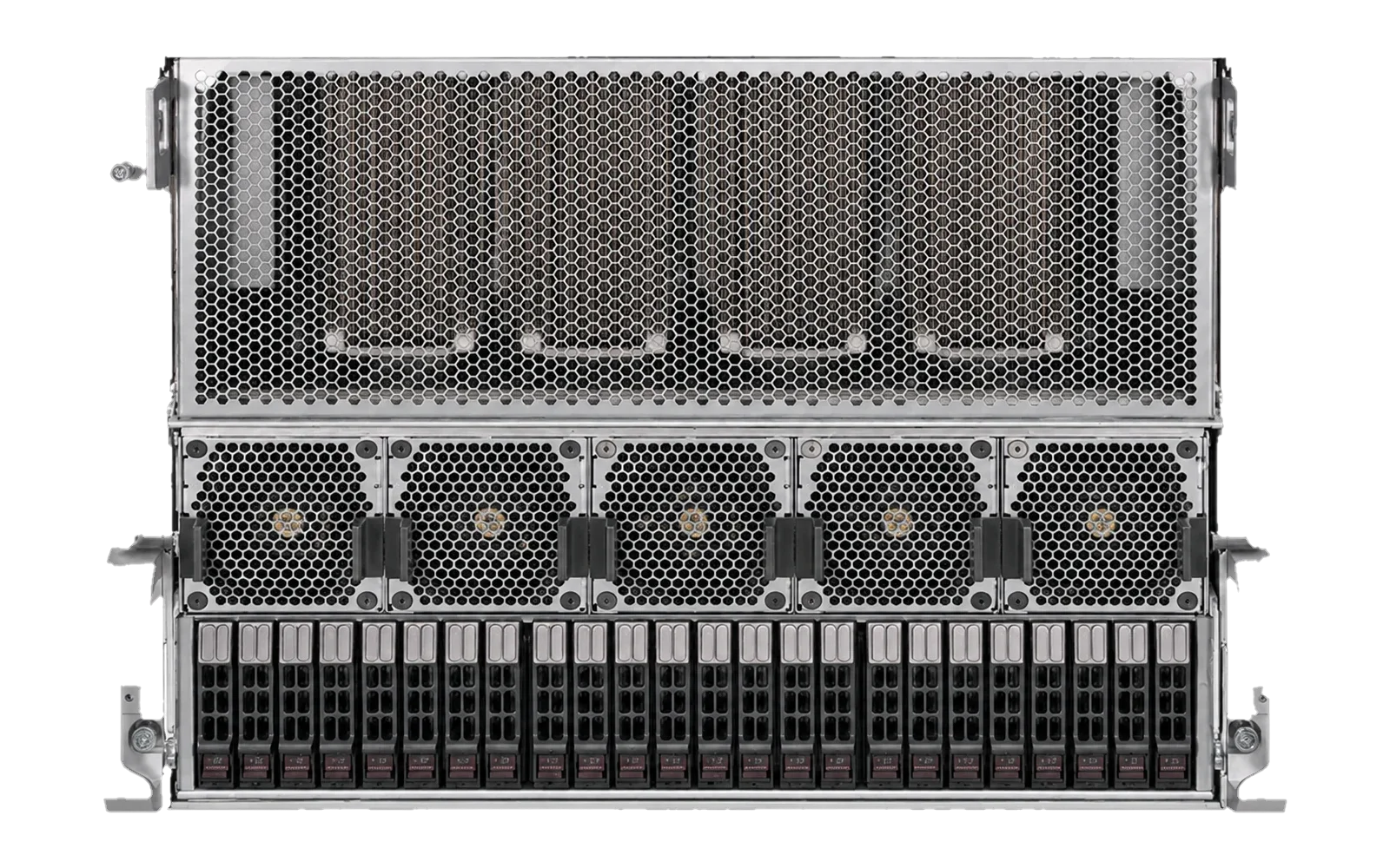
When a workload belongs on controlled infrastructure, xSONiC can size an 8-GPU AI Inference Server together with networking, NVMe storage, observability, site readiness, and handover. The configuration is selected from the target models and request profile, then validated with measured throughput and latency rather than a generic benchmark.
FAQ
Frequently asked questions
Is self-hosting an LLM cheaper than using a cloud API?
It depends on volume, utilisation, and operating cost. Low or irregular usage usually favours metered APIs. Steady high usage can favour owned capacity when hardware, power, cooling, rack space, support, and operations are included in the comparison.
Are open models suitable for enterprise workloads?
Open models can suit retrieval-grounded assistants, summarisation, coding, document processing, and internal APIs, but suitability is task-specific. Evaluate candidate models on representative data and quality criteria before selecting an architecture.
Can an organisation combine cloud AI and self-hosted LLMs?
Yes. A common design keeps experiments, short-lived peaks, and workloads that require closed models in the cloud while routing steady or sensitive workloads to private infrastructure behind the same internal service interface.
What is the minimum hardware for production self-hosting?
There is no universal minimum. The starting configuration follows model memory, precision, context length, concurrency, latency, availability, and growth requirements. Small GPU systems can support evaluation, while production services should be sized from a measured request profile.
Continue reading
Related articles
 Technical ArticleNetwork and Storage Planning for Private AI Inference Servers: A Practical Buyer GuideA practical buyer guide to network and storage planning for private AI inference servers in Australian data centers.Read article
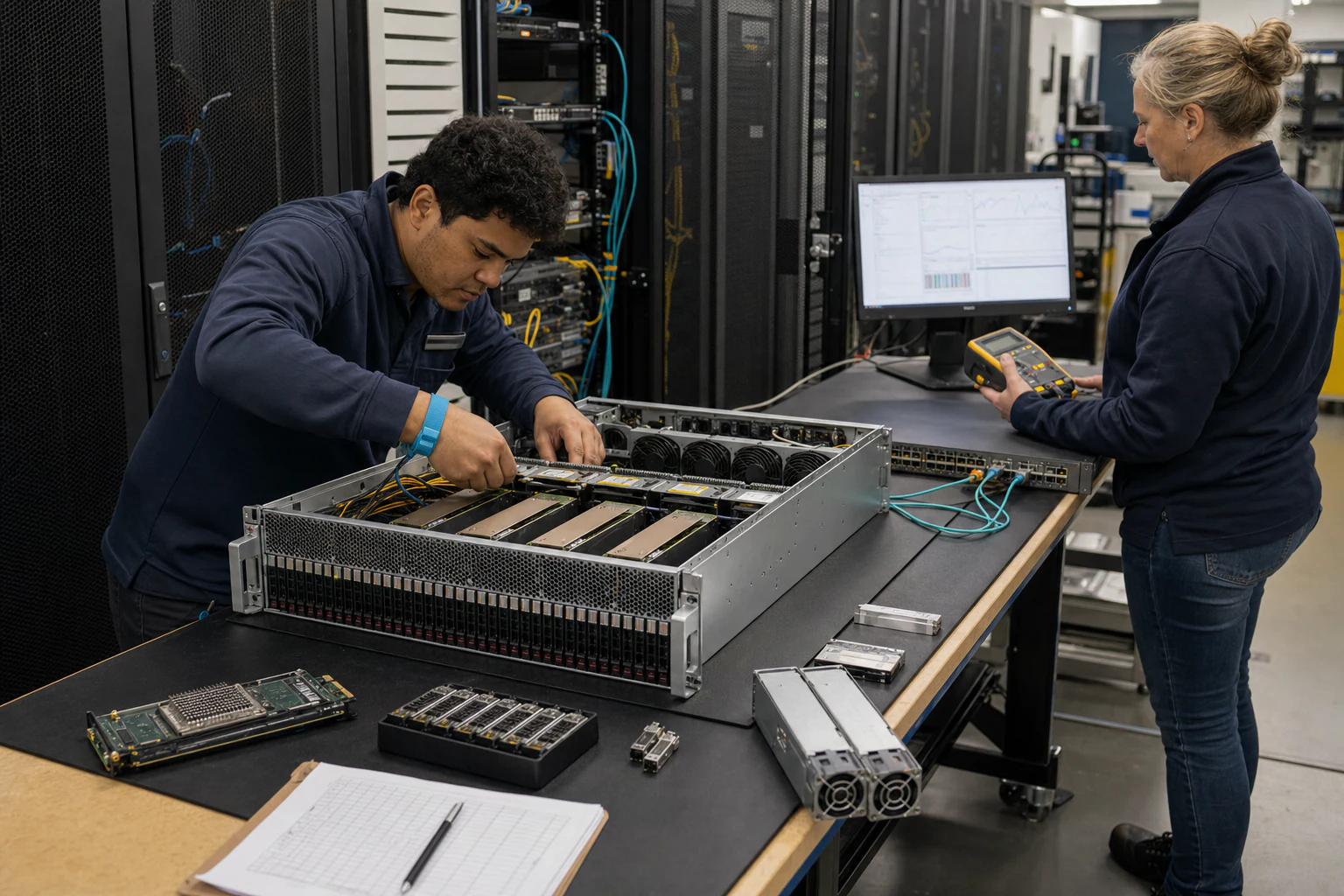 Technical ArticleProcurement Scorecard: Networking Infrastructure for Private AI Inference in Australian Enterprise ProgramsEngineering guidance on Procurement Scorecard for Australian infrastructure teams, covering form factor tradeoffs, capacity planning, thermal design, endurance, and.Read article
 Technical ArticlePrivate AI Inference Networking in Australia: What Enterprise GPU Deployments Need from the Network LayerEngineering guidance on Private AI Inference Networking in Australia for Australian network teams, covering underlay design, EVPN-VXLAN operations, interoperability.Read article
Relevant hardware
Related products
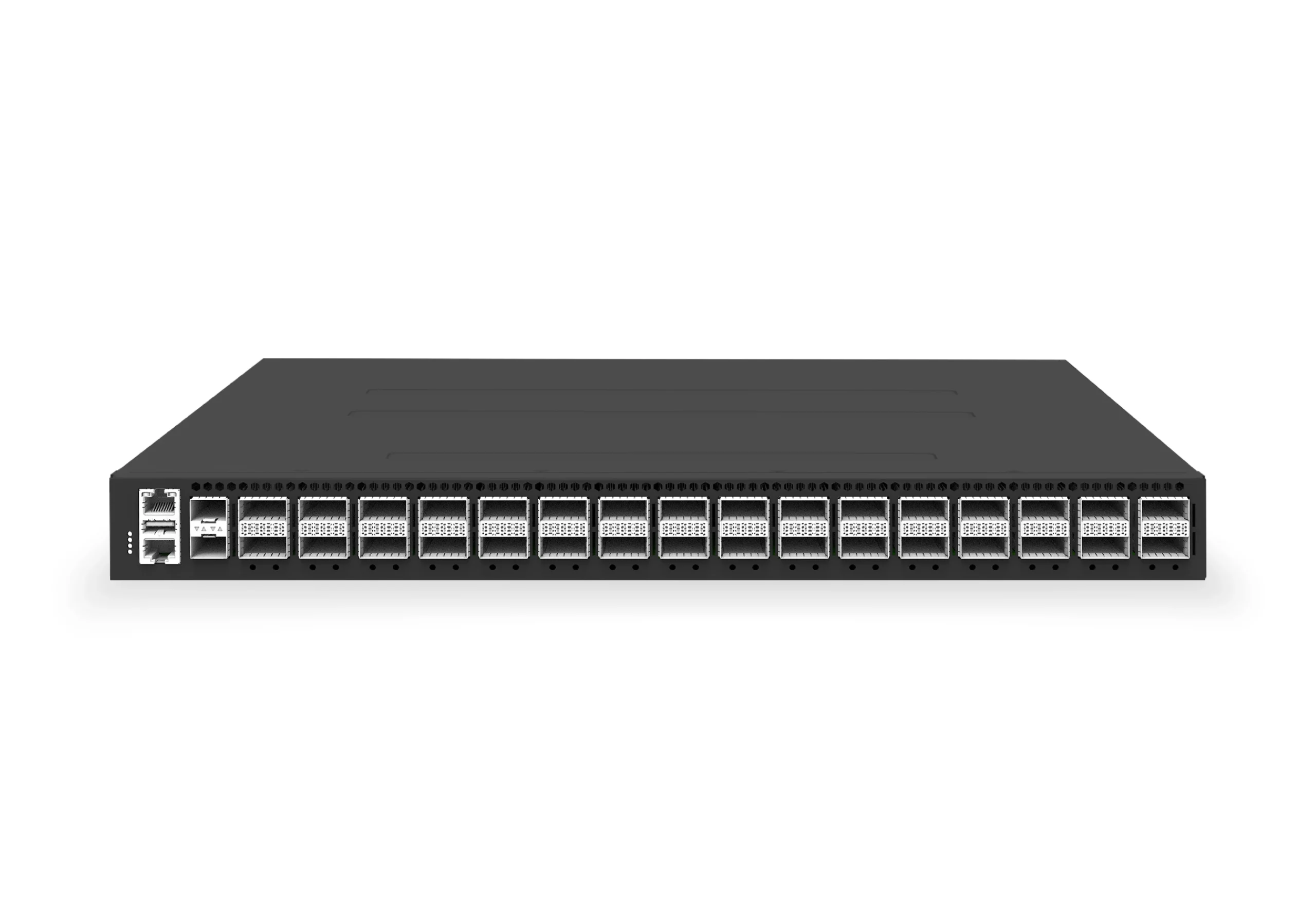 datacenter aiXS-DC-32X400-SP-G232-port 400G spine/core switch for high-capacity data center fabrics and AI-ready backbones.View product
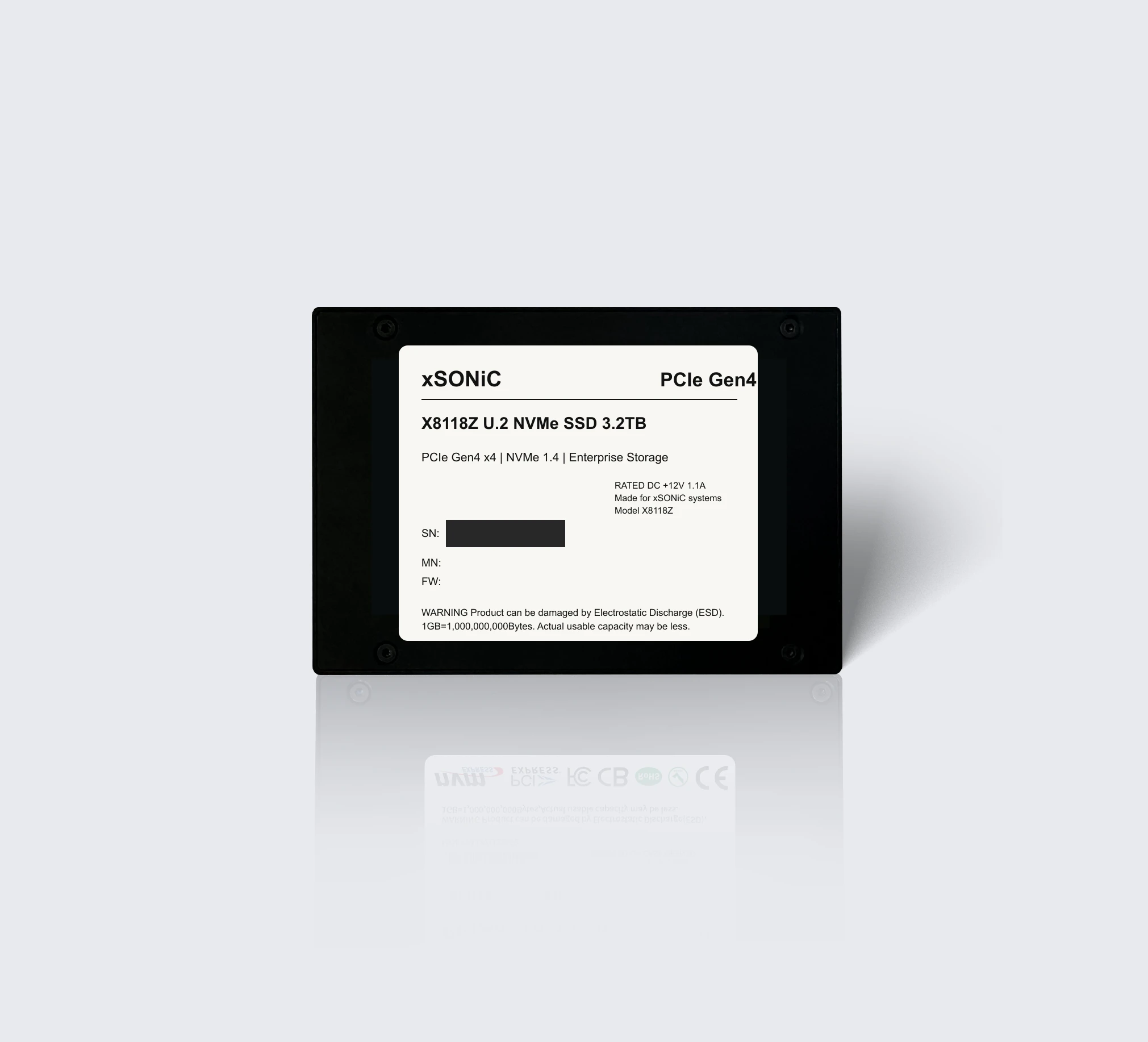 nvme ssdXS-SSD-8118Z-U2Enterprise U.2 NVMe SSD with PCIe Gen4 x4, NVMe 1.4, up to 7.1 GB/s sequential read, and 1,000K IOPS for data center storage workloads.View product