Why Tokens-per-Second Benchmarks Mislead LLM Infrastructure Buyers

In brief

A single tokens-per-second figure cannot predict an LLM service. The result changes with the exact model, precision, prompt and output distribution, batching, serving framework, and latency constraint. A useful benchmark pins those conditions to the intended workload, reports p50 and p95 latency beside sustained throughput, and is refreshed whenever the model or serving stack materially changes.

Key takeaways

• A token-rate result without its model, precision, context profile, and latency condition is not comparable.
• Batching can raise aggregate throughput while making each request wait longer, so throughput and latency must be reported together.
• Prefill and decode stress different parts of the system; the prompt-to-output ratio changes the bottleneck.
• Framework, driver, kernel, firmware, and serving parameters belong in the result because software releases can move performance.
• Public benchmarks help shortlist platforms; production sizing still requires measurement on the target workload and intended system.

Tokens per second looks like an ideal buying metric: one unit, one number, and an intuitive assumption that bigger is better. It is not a specification of an LLM service. It is the outcome of one model, one request mix, one software stack, one load level, and one measurement boundary.

A token generated by a small quantised checkpoint after a short prompt is not the same systems job as a token generated by a larger model after a long RAG context. Even the phrase “tokens per second” may mean output tokens from one request, aggregate output across a server, or input and output tokens combined. All three numbers can be calculated correctly and still answer different questions.

For a private-inference buyer, the useful question is: how many representative requests can this complete while meeting our latency, quality, availability, power, and data-boundary requirements? The rest of this guide turns that question into a repeatable sizing and acceptance test.

Why the Same Appliance Produces Different Headline Numbers

Keep the physical server unchanged and alter the checkpoint, weight or KV-cache datatype, prompt length, output length, batch policy, prefix-cache hit rate, or serving release. The measured rate moves. Increase offered load until every accelerator is saturated and aggregate throughput may rise further, even while users wait longer in a queue.

That does not automatically make a vendor result dishonest. An offline test is useful for an overnight summarisation queue. A latency-free saturation number is simply not evidence for an interactive assistant. The opposite distortion also occurs: a cold compile, unsuitable kernel, client bottleneck, storage contention, or conservative scheduler can make capable hardware appear slow.

Treat every result as a statement about a system under test and a workload, not as a permanent property of an accelerator or appliance.

Use a Complete LLM Inference Vocabulary

Define each timing boundary before comparing reports. For procurement, client- observed measurements are usually the most useful because they include the service path a user actually experiences.

Metric	Precise meaning	Buying use
TTFT — time to first token	Time from client submission to receipt of the first non-empty output token. At this boundary it includes gateway and network time, queueing, tokenisation, prefill, and first-token delivery.	Responsiveness of chat, search, and RAG. Report p50, p95, and preferably p99. Label engine-only TTFT separately.
TPOT — time per output token	For one completed request with more than one output token: (end-to-end latency - TTFT) / (output tokens - 1). It is an average decode interval for that request.	Smoothness of generation and a useful inverse of single-request decode rate. It can hide individual stalls.
ITL — inter-token latency	The observed interval between each pair of consecutive streamed output tokens. Aggregate the intervals with an explicitly stated method.	Reveals pauses that per-request TPOT averages can conceal. Report its distribution, not only the mean.
E2E latency	Time from client submission until the final output token or complete non-streamed response is received.	Completion time experienced by applications and users. It depends on both output length and service delay.
Request throughput	Successfully completed requests divided by measured wall time.	Capacity when requests are sufficiently comparable and their length distribution is fixed.
Output-token throughput	Successfully returned output tokens divided by measured wall time, normally aggregated across the system.	Decode-heavy capacity. State whether cancelled and partial requests are counted.
Concurrency	Number of requests in flight. It is a population, not an arrival rate.	Exposes queueing, scheduling, and KV-cache capacity. The same concurrency can represent different RPS at different latencies.
Goodput	Requests per second, or tokens per second, that satisfy every stated SLO and quality rule. The unit and pass rule must be explicit.	The most decision-useful capacity metric because late, failed, or unacceptable responses do not become useful work.

“Total tokens per second” often adds prompt and output tokens. That can be useful for an engine study, but it combines prefill and decode work with very different characteristics. Do not compare it with output-only TPS. Likewise, do not convert an average TPOT into a fleet-capacity promise: continuous batching means aggregate server throughput is not simply the reciprocal of one request’s TPOT.

Goodput prevents a common benchmark failure. If a server accepts more traffic but breaches the p95 TTFT or TPOT target, its raw throughput increased while its usable capacity did not. Define whether goodput is counted per request or per output token and require, for example, that a request pass all TTFT, TPOT, E2E, completion, and quality gates before it contributes.

Prefill, Decode, and the KV Cache Explain the Trade-offs

LLM inference contains two materially different phases.

Prefill processes the complete input sequence and creates attention state for it. Prompt tokens can be processed in parallel, so prefill tends to make strong use of matrix-compute capability. Longer system prompts and retrieved documents therefore increase TTFT even when the requested answer is short.

Decode is autoregressive: each new token depends on the preceding context. The engine repeatedly accesses model weights and the request’s stored attention state. Decode at modest batch sizes is commonly sensitive to memory bandwidth, while continuous batching and higher concurrency can improve utilisation at the cost of queueing or token-to-token delay.

The KV cache stores key and value activations created for prior tokens so the model does not recompute the entire history at every decode step. Its size grows with active sequence length and request count, and also depends on model architecture, attention layers and heads, tensor parallelism, and cache datatype. Model weights fitting in accelerator memory does not prove that the production concurrency and context lengths will fit.

Paged allocation, as described in the PagedAttention work behind vLLM, reduces allocation waste and fragmentation and enables more flexible sharing. It does not make the physical state for unique tokens free. Under cache pressure, an engine may queue, evict, pre-empt, recompute, offload, or reject work; each choice can change tail latency. Record cache utilisation, pre-emption or recompute counts, and rejected requests beside TPS.

Scheduler settings matter too. Chunked prefill can split a long prompt so decode work is not blocked behind one large prefill. The chosen token budget then trades TTFT against ITL. Prefix caching can help workloads with genuinely repeated prefixes, but a benchmark must state cache state, hit ratio, eviction policy, and whether each run began warm or empty. An artificial 100 percent hit rate is not representative evidence unless production really has one.

Define the Workload Before Selecting Hardware

The workload definition should be an attachment to the request for quotation, not a conversation after delivery.

Condition	Minimum reproducibility record
Model and task	Repository or source, exact checkpoint and revision, architecture, tokenizer revision, chat template, context limit, and any adapters
Numerical format	Weight, activation, and KV-cache datatypes; quantisation algorithm and calibration; tensor, pipeline, data, or expert parallel layout
Generation policy	Temperature, top-p/top-k, beam or speculative settings, stop rules, maximum new tokens, and whether EOS is honoured
Request distribution	Histograms or percentiles for input tokens, requested and actual output tokens, active context, turns per session, modalities, and cancellation rate
Arrival pattern	Open-loop request rate or timestamped trace, burst distribution, planned and stress concurrency, queue and admission limits
Service path	Client location, TLS and gateway path, authentication, API compatibility, streaming mode, retrieval dependency, and response post-processing
Software and hardware	Appliance BOM and topology, firmware, OS, driver or ROCm release, framework build or container digest, kernels, and material flags
Acceptance gates	Quality dataset and threshold, TTFT/TPOT/ITL/E2E percentiles, errors, timeouts, goodput unit, run length, repeatability, and power boundary

Use production traces after removing sensitive content where governance permits. If no trace exists, create several declared profiles rather than one average. Tokenise with the exact production tokenizer: character count and word count are not reliable substitutes. Preserve the long tail because a small fraction of large contexts can dominate KV-cache use and p95 latency.

Quality is part of the workload. Quantisation, speculative decoding, or a different checkpoint may improve speed but alter outputs. If a configuration fails the agreed task-level evaluation, it is a different service rather than a faster implementation of the accepted one.

Build a Test Matrix That Exposes the Bottleneck

At minimum, cross each representative profile with low, planned, peak, and overload arrival levels. Run both normal and adverse infrastructure conditions that are in operational scope.

Profile	Primary pressure	Required observations
Short interactive chat	Queueing and decode responsiveness	TTFT, TPOT and ITL percentiles, goodput, session concurrency
Long-context RAG, short answer	Prefill, KV cache, retrieval and network	Retrieval-only latency, model TTFT, E2E latency, input-token rate, cache pressure
Coding or report generation	Long decode and cancellation behaviour	Output TPS, TPOT/ITL, E2E by output-length bucket, cancelled work
Mixed production trace	Scheduler fairness and length interference	Per-profile and combined percentiles, queue depth, errors, starvation
Offline generation	Sustained saturation and job completion	Output tokens/hour, jobs/hour, energy per completed unit, retries
Model load or failover	Storage, readiness and resilience	Load/warm-up time, health transition, recovery, capacity during loss of a worker

Do not let the shortest profile hide the longest. Report every profile separately as well as the mix.

A Reproducible Benchmark Runbook

1. Freeze the acceptance definition

Give the run a unique ID. Hash or record the dataset, checkpoint, tokenizer, quality set, configuration, container image, and test script. Capture the appliance serialised BOM, accelerator topology, firmware, power mode, CPU/NUMA binding, network links, and storage path. Synchronise client and server clocks, but compute client-observed intervals from one monotonic clock.

2. Separate cold-start and steady-state tests

Measure model download or read, engine initialisation, compilation, cache allocation, readiness, and first successful request as an operational test. Then perform declared warm-up requests before the steady-state performance run. Never blend cold-start samples into warm results or quietly discard them.

3. Validate the generator and a single-request baseline

Run the load generator on a separate, adequately sized host when possible. Confirm that its CPU, NIC, connection pool, TLS stack, and tokenisation are not the bottleneck. At concurrency one, verify response correctness, token counts, stop behaviour, streaming timestamps, and the measurement boundary. This is a sanity check, not the capacity result.

4. Replay the distribution and sweep offered load

For an online service, prefer an open-loop arrival process or timestamped trace. A closed-loop client that waits for each response before issuing another request reduces its own offered load when the server slows, concealing overload. Sweep request rate through the expected operating range and beyond the knee where queues and tail latency rise. Repeat each point with fixed seeds and a consistent cache policy.

Current vLLM releases provide a serve benchmark with request-rate, burstiness, concurrency, percentile, detailed-result, and goodput controls. A version-pinned invocation can follow this pattern; substitute the values from the test plan and archive the resolved command because CLI defaults change:

vllm bench serve \
  --base-url "$ENDPOINT" \
  --model "$MODEL_ID" \
  --dataset-name custom \
  --dataset-path "$TRACE_JSONL" \
  --request-rate "$REQUESTS_PER_SECOND" \
  --max-concurrency "$CONCURRENCY_CAP" \
  --num-prompts "$REQUEST_COUNT" \
  --seed "$SEED" \
  --percentile-metrics ttft,tpot,itl,e2el \
  --metric-percentiles 50,95,99 \
  --goodput "ttft:$TTFT_SLO_MS" "tpot:$TPOT_SLO_MS" "e2el:$E2E_SLO_MS" \
  --save-result --save-detailed \
  --metadata "image_digest=$IMAGE_DIGEST" "run_id=$RUN_ID"

The tool is not the methodology. Confirm its metric formulas and client timing against the pinned release. Preserve raw per-request data so a reviewer can recalculate percentiles and inspect failures rather than trusting a console summary.

5. Observe the complete system for long enough

Continue measured steady state until temperatures, clocks, power, cache use, queue depth, and throughput have stabilised and there are enough samples for the required tail percentile. Record duration and sample count; do not assume a brief burst represents continuous operation. Repeat runs and report the median plus range or confidence interval, not only the best attempt.

Collect client request timestamps and status, actual input/output token counts, server queue and scheduler metrics, KV-cache occupancy and pre-emption, CPU and accelerator utilisation, memory, clocks, temperature, error logs, NIC traffic, storage activity, and power. Correlate them on the run timeline.

6. Re-run quality and failure cases

Evaluate outputs produced by the same configuration used for performance. Test a burst above the admission limit, maximum supported context, malformed and cancelled requests, dependency delay, a worker or link loss where supported, and recovery to readiness. Acceptance should specify whether excess traffic is rejected promptly or queued within a bounded time; an appliance that merely accumulates an unbounded queue has not preserved service.

Measurement Pitfalls That Create Attractive but Useless Results

• All requests at time zero: this is an offline saturation pattern, not an interactive arrival process. Label it as offline throughput.
• Fixed short prompts or outputs: they omit long-context cache pressure and can overstate capacity for a mixed service.
• Forcing a fixed generation length: ignoring EOS makes token counts tidy but changes work and user behaviour. If used, disclose it and run a realistic stop-policy test too.
• A warm prefix cache with no hit-rate disclosure: repeated synthetic prompts can avoid prefill work that production must perform.
• A client-side bottleneck: an underpowered generator may report a flat throughput curve and falsely attribute the ceiling to the server.
• Inconsistent token accounting: server and client tokenisers or chat templates can disagree. Save exact token IDs or counts at the chosen boundary.
• Averages of averages: calculate percentiles from raw requests at each run point. Do not average vendor p95 values or pool unlike workload profiles.
• Dropping failures and cancellations: disclose offered, accepted, completed, failed, timed-out, rejected, and cancelled requests. Goodput must not reward incomplete work.
• Changing several variables together: a new driver plus new quantisation plus different scheduler cannot identify which change caused the result.
• Cherry-picking the fastest run: show repetitions and variance, including thermal or cache-pressure degradation.

Power, Thermals, Network, and Storage Are Part of the Appliance

Component telemetry is useful for diagnosis, but procurement should also measure AC energy at the appliance or rack power boundary. Report average and peak power during the same accepted run, energy per SLO-passing request or per valid output token, and idle power. Record the power cap, fan policy, inlet temperature, ambient conditions, PSU configuration, and whether redundant power was active. A result obtained before temperature and clocks stabilise is not a sustained rating.

Verify the facility can supply and remove the measured load with the intended redundancy and headroom. Watch for power or thermal throttling on a timeline; average accelerator utilisation alone will not explain it.

Place the load generator so its link does not compete unintentionally with model loading, storage, or retrieval traffic. Record negotiated link speed, errors, retransmissions, drops, gateway CPU, and payload volume. For RAG, report retrieval latency separately and also measure full application E2E latency. For model operations, test read or transfer time from the intended repository, local storage, or network path. The private-AI network and storage planning guide covers those dependencies in more detail.

Worked Sizing Example: From Requirement to Evidence

Consider an internal RAG assistant. The following values are illustrative requirements, not platform results. The buyer has a sanitised trace containing short chat turns and long document questions, defines its exact model and quality set, and requires p95 TTFT, TPOT, and E2E limits plus a completion and error-rate gate. It also forecasts a peak arrival rate and a growth factor.

The team replays the trace at increasing open-loop RPS. At every load point, a request counts toward request goodput only if it completes, passes the quality rule, and meets all latency SLOs. The accepted capacity is the highest repeated load at which every service gate remains satisfied; the first higher point should demonstrate predictable queueing or rejection rather than hidden failure.

Sizing then uses measured accepted capacity:

required active appliances = ceil((forecast peak RPS × growth and operating headroom) / measured goodput per appliance)

Redundancy is applied after that calculation. Re-run the matrix with one worker or appliance unavailable to prove the intended failover policy. Do not divide peak demand by brochure TPS, and do not infer the required fleet from average output length alone. Cache capacity, request mix, and latency gates are already captured in measured goodput.

Turn the Test Into Contractual Acceptance Criteria

A useful acceptance schedule states pass/fail rules before hardware arrives.

Acceptance area	Example of a measurable rule structure
Identity	Delivered BOM, topology, firmware, model revision, numerical format, container digest, and configuration match the approved baseline
Quality	Same performance configuration meets the agreed task-level dataset and threshold
Interactive service	At each required trace and offered-load point, p50/p95/p99 TTFT, TPOT/ITL, and E2E remain within named limits
Capacity	Repeated request goodput meets or exceeds required peak plus stated operating headroom; raw throughput is reported but is not the pass metric
Reliability	Completion, timeout, rejection, and server-error rates remain within limits; overload and recovery behaviour match policy
Memory	Maximum supported context and planned concurrency complete without unapproved cache offload, repeated pre-emption, or out-of-memory failure
Sustained operation	A declared steady-state duration passes without material throughput loss, clock throttling, thermal alarm, or error accumulation
Infrastructure	Wall power, energy, inlet temperature, NIC and storage results remain within facility and design limits
Repeatability	Required repetitions stay within an agreed variance and all scripts, configurations, logs, and raw results are delivered

Specify refresh triggers as well: model or tokenizer revision, quantisation, driver or ROCm stack, firmware, serving framework, scheduler policy, context distribution, concurrency target, security gateway, and storage or network path. A benchmark is dated evidence; material changes create a new system under test.

Procurement Checklist

Before comparing AI inference appliances, ask each supplier for:

• the exact checkpoint, revision, tokenizer, precision, quantisation and quality result used for every performance claim;
• raw input/output length distributions, arrival process, cache policy, concurrency sweep, warm-up, duration, repetitions, and random seeds;
• client-observed TTFT, TPOT, ITL and E2E percentiles beside request throughput, output TPS, goodput, errors, timeouts, rejections, and cancellations;
• the complete hardware topology and software/firmware bill of materials, container digest, launch command, environment, and benchmark scripts;
• KV-cache allocation and peak use, pre-emption/recompute behaviour, maximum tested context, and evidence for planned concurrency;
• sustained wall power and energy, thermals and clocks, plus NIC, storage and retrieval observations collected during the accepted run;
• cold load, warm-up, overload, failover, restart and recovery results;
• a right to repeat the agreed test on the delivered system and a process for revalidation after material software or model changes.

If a result omits its latency constraint, workload distribution, or failure count, it is a lead for further testing rather than procurement evidence.

Minimum Result Template

Every submitted result should contain one row per workload and load point, with raw files attached:

Section	Required fields
Run identity	Run ID, timestamp, operator, commit/script hash, dataset hash, seed
Workload	Model/revision, tokenizer/template, datatypes, quality score, input/output/context percentiles, arrival profile
System	Appliance BOM and topology, firmware, OS, driver/ROCm, framework/container digest, configuration and cache state
Method	Client path, warm-up, duration, sample count, offered RPS, concurrency/admission policy, repetitions
Service result	Accepted/completed/failed/timed-out/rejected/cancelled counts; TTFT, TPOT, ITL and E2E p50/p95/p99; request and token throughput; goodput
Resource result	KV-cache peak and pre-emption, memory/utilisation, clocks, temperatures, AC power/energy, NIC and storage peaks
Decision	Pass/fail by gate, variance across repeats, limitations, approver, and refresh triggers

Use Public Benchmarks to Shortlist, Then Validate the Workload

MLPerf Inference demonstrates valuable discipline: a defined system under test, scenario-specific load generation, latency and quality constraints, required disclosures, and reproducibility rules. Current public results can help identify candidate platforms and software progress within comparable categories. They do not model every private RAG trace, network path, quantisation choice, or latency promise.

xSONiC therefore does not treat one generic TPS headline as a permanent specification of the AI Inference Server. Sizing and validation should use the intended checkpoint, numerical format, request distribution, software release, infrastructure path, and acceptance gates. The deliverable is not just a fast number; it is a reproducible result, an operating boundary, and evidence that the purchased service meets its users’ requirements.

Product fit

Where xSONiC Fits

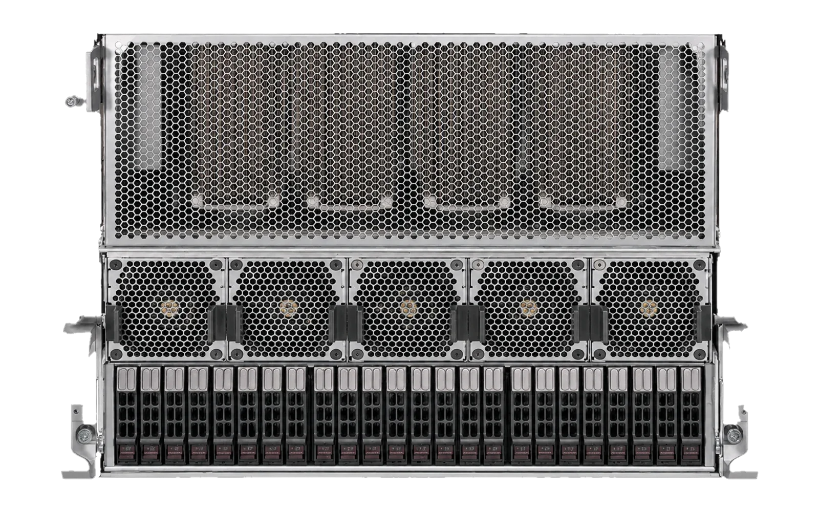
xSONiC sizes and validates the AI Inference Server against the customer's exact checkpoint, precision, request distribution, concurrency, and latency target. Results are reported with their software versions and test conditions so they can be reviewed and repeated rather than treated as a permanent generic platform number.

ai infrastructurexSONiC AI Inference ServerPrivate AI inference platform for local LLM, RAG, coding, document intelligence, and multimodal services, with xSONiC deployment support across compute, network, storage, and validation.View product→

FAQ

Frequently asked questions

What is a good tokens-per-second result?

It depends on the exact checkpoint, precision, prompt and output lengths, concurrency, serving framework, and p95 latency target. A good result is the sustained throughput that meets the application's quality and latency requirements under a representative request distribution.

Why can vendor benchmark numbers exceed production results?

A published test may use a smaller model, lower precision, shorter contexts, aggressive batching, a tuned software release, or no user-facing latency constraint. Those conditions can be legitimate, but they may not represent the buyer's workload. Ask for the complete test definition before comparing results.

Why report p95 latency with throughput?

p95 describes the latency that 95 percent of measured requests meet or beat. It exposes tail behaviour that averages can hide and constrains how aggressively a service can batch requests. Throughput without its p95 condition does not show the user experience at that load.

How long should an inference benchmark run?

Long enough to include warm steady state, repeated samples, planned and stress concurrency, realistic context variation, and any thermal, queueing, or memory behaviour that short bursts hide. Report duration, warm-up, repetitions, ranges, and failure criteria instead of relying on one run.

Continue reading

Related articles

Technical ArticleNetwork and Storage Planning for Private AI Inference Servers: A Practical Buyer GuideA practical buyer guide to network and storage planning for private AI inference servers in Australian data centers.Read article→

Technical ArticleWhat a GPU Actually Does and Why Your Network Fabric Determines Its Real PerformanceEngineering guidance on a GPU Actually Does and Why Your Network Fabric Determines Its Real Performance for Australian network and security teams, covering traffic.Read article→

Technical ArticlePrivate AI Inference Is Reshaping Data Center Networking - And Australian Enterprises Are Starting to Pay AttentionEngineering guide to private AI inference networking for Australian enterprises, covering SONiC, RoCE, NVMe-oF, GPUDirect Storage, telemetry, and sovereignty.Read article→